In this article, we will explore Database Indexing. We will begin by installing the Docker & running a Postgres container on it. Subsequently, to execute queries and comprehend how the database uses various indexing strategies, we will insert millions of rows into a Postgres table.
Following that, we will explore different tools to gaining insights into the SQL query planner and optimizers. After that, we will delve into understanding database indexing, examining how various types of indexing works with examples, and do a comparison between different types of database scan strategies.
Finally, we will then demystify how database indexes operates for the WHERE clause with the AND and OR operators.
Prerequisite
Installing Docker & Running a Postgres Container:
Install Docker by following the instructions provided in the getting started guide on the official Docker website.
Verify that Docker is installed by running the command docker --version
Running a PostgresSQL Container:
Spin up the Docker container by using the official Postgres image.
docker run -e POSTGRES_PASSWORD=secret --name pg postgres
This sequence of steps creates a table named employees and inserts one million rows into it, generating random values for the employeeid and name columns. The final count query verifies the successful insertion of the specified number of rows.
The SQL Query Planner and Optimizer:
Explanation:
The explain command displays the execution plan generated by the PostgresSQL planner for the provided statement. This plan illustrates how the table(s) referenced in the statement will be scanned, whether through plain sequential scans, index scans, etc.
Seq Scan: Directly goes to the heap and fetches everything, similar to a Full Table Scan in other databases. In Postgres, with multiple threads, it's called Parallel Seq Scan.
Cost=0.00..16139.01: The first number represents work before fetching (e.g., aggregating, ordering), and the second number is the total estimated execution time.
rows=1000001: An approximate number of rows to be fetched.
rows=1: Fetching only 1 record using the primary key index.
What is Database indexing?
An index is a data structure that speeds up data retrieval without needing to scan every row present in the table. Index improves lookup performance but decreases write performance because every time a new row is created, indexes need to be updated.
Indexes are typically stored on the disk. An index is typically a small table with two columns: a primary/candidate key and address. Keys are made from one or more columns.
The data structure used for storing the index is B+ Trees. In the simplest form, an index is a stored table of key-value pairs that allows searches to be conducted in O(logn) time using binary search on sorted data.
Types of Indexes:
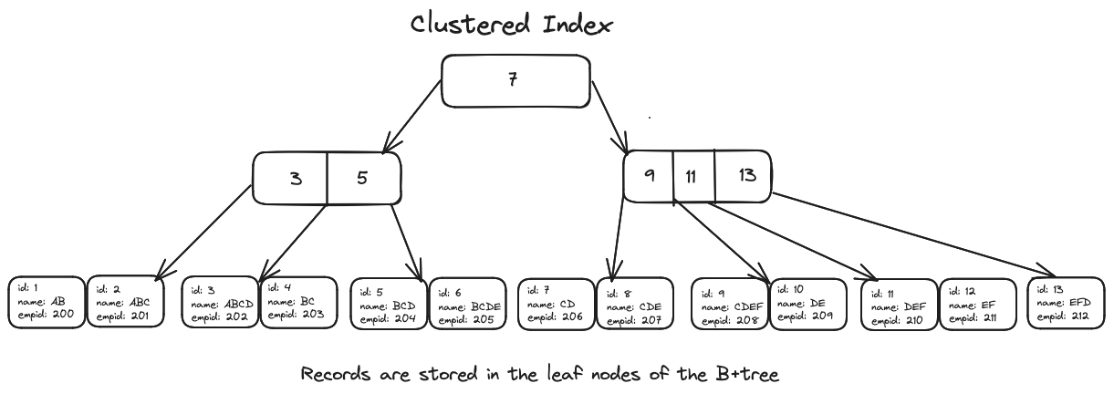
Clustered Index
Index and data reside together and are ordered by the key. A Clustered Index is basically a tree-organized table. Instead of storing the records in an unsorted Heap table space, the clustered index is actually B+Tree index having the Leaf Nodes, which are ordered by the clusters key column value, store the actual table records, as illustrated by the following diagram.
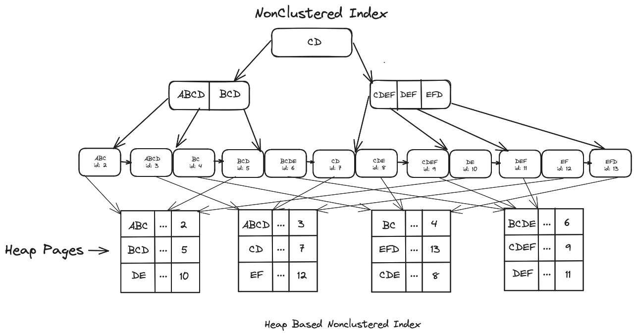
Nonclustered Index
A nonclustered index contains the key values and each key value entry has a pointer to the data row that contains the key value. Since the Clustered Index is usually built using the Primary Key column values, if you want to speed up queries that use some other column, then you'll have to add a Secondary Non-Clustered Index.
The Secondary Index is going to store the Primary Key value in its Leaf Nodes, as illustrated by the following diagram
How database indexes works under the hood?
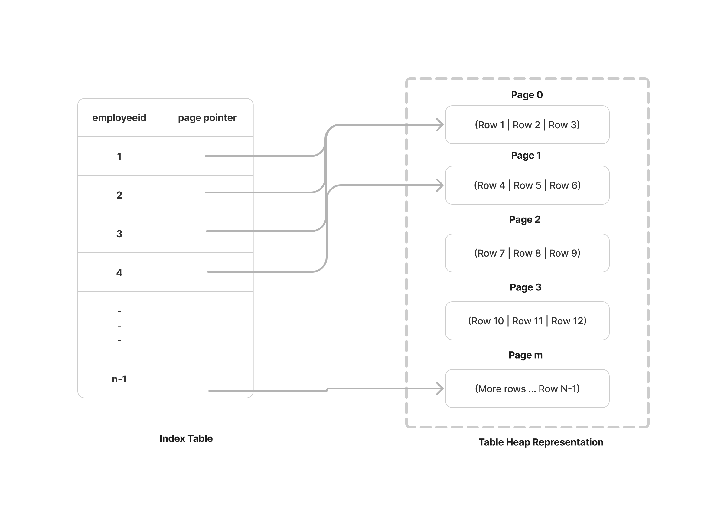
We have already created a database index on the employeeid column in our employees table using the CREATE INDEX statement. Behind the scenes, Postgres creates a new pseudo-table in the database with two columns: a value for employeeid and a pointer to the corresponding record in the employees table. This pseudo-table is organized and stored as a binary tree with ordered values for the employeeid column. Consequently, the query operates with O(logn) efficiency and typically executes in a second or less.
Let’s delve into two scenarios:
SELECT * FROM employees WHERE employeeid = 4;
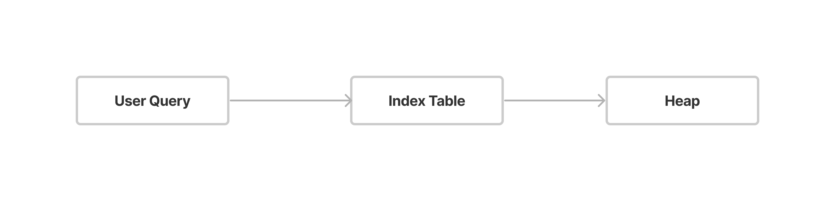
Here, with an index on the employeeid column, the query initiates an Index Scan. The process begins by accessing the Index table, retrieving the reference for the Page number, and obtaining the row number for the specific record on that page. Subsequently, it navigates to the corresponding page in the heap and fetches the entire row. This method, known as an Index Scan.
SELECT employeeid FROM employees WHERE employeeid = 4;
In this instance, there is no need to access the heap to retrieve the complete record. Since the required value for employeeid is already present in the index table, the operation is streamlined, and it directly performs an Index Only Scan. This approach allows the system to retrieve the specific employeeid directly from the index table without the additional step of fetching the complete row from the heap. This can lead to improved performance, particularly when the index includes all the columns needed for the query, minimizing the amount of data that needs to be processed.
What are different type of database scan strategies?
If we examine the given query, we retrieve the ID using a filter on the ID column, which serves as the primary key and has an index on it.
Let's break down the query output:
Index Only Scan: In the case of an Index Only Scan, Postgres scans the index table, resulting in faster performance as the Index table is significantly smaller than the actual table. With Index Only Scan, results are directly fetched from the Index table when querying columns for which indexes have been created.
Heap Fetches: 0: This indicates that the queried ID value did not necessitate accessing the heap table to retrieve information. The information was obtained inline, and this is referred to as an Inline query.
Planning Time: 0.510 ms: This represents the time taken by Postgres to determine whether to use the index or perform a full table scan.
Execution Time: 2.708 ms: This is the time taken by Postgres to actually fetch the records from the table.
If we examine the given query, we are retrieving the name using a filter on the ID column, which serves as the primary key and has an index on it.
In this case, the process begins with an index scan on the Index table to retrieve information about the Page number and row number on the Heap. Since the name is not available in the Index table, we must go to the heap to fetch the name. This type of scan is referred to as an Index Scan.
In this case, we are filtering the record using the filter on the id with '<' operator and filtering out record which have id less than 1000. So the process begins with an Index scanning on the Index table then fetching the rows from the heap. Same as in case of fetching single id.
In this case, we are filtering the record using the filter on the id with '>' operator and filtering out records which have id greater than 1000. So, in this case, as Postgres knows it has to fetch 99% of the data anyway, it prefers to use the Seq Scan on the heap table. Rather than going to the Index table to filter out the records and then again going to the heap to filter those Index-scanned rows.
If we examine the given query, we are retrieving the id using a filter on the name column, which doesn't have an index on it.
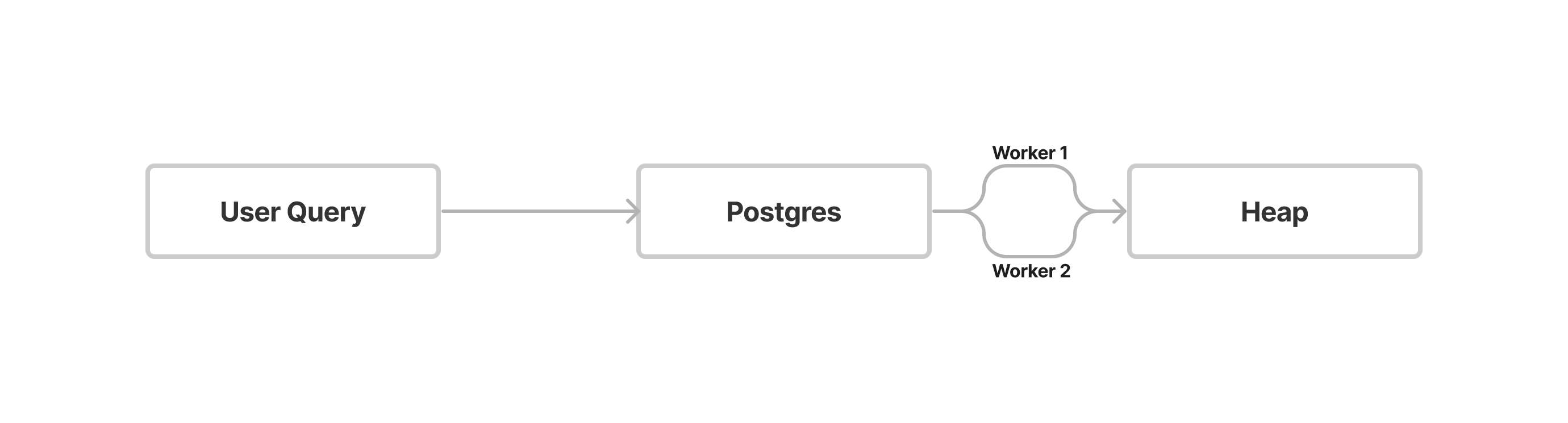
As we don't have an index on the name column, that means we have to actually search for the name WABOY one by one and perform a sequential scan on the employees table. Postgres efficiently addresses this by executing multiple worker threads and conducting a parallel sequential scan.
Bitmap Scan
Let's create a Bitmap Index on the name column to get started.
Let's explore how Bitmap Scan works in PostgreSQL.
Heap pages are stored on disk, and loading a page into memory can be expensive. When using an Index Scan, if the query yields a large number of rows, the query's performance may suffer because each row's retrieval involves loading a page into memory.
In contrast, with a Bitmap Scan, instead of loading rows into memory, we set a bit to 1 in an array of bits corresponding to heap page numbers. The operation then works on top of this bitmap.
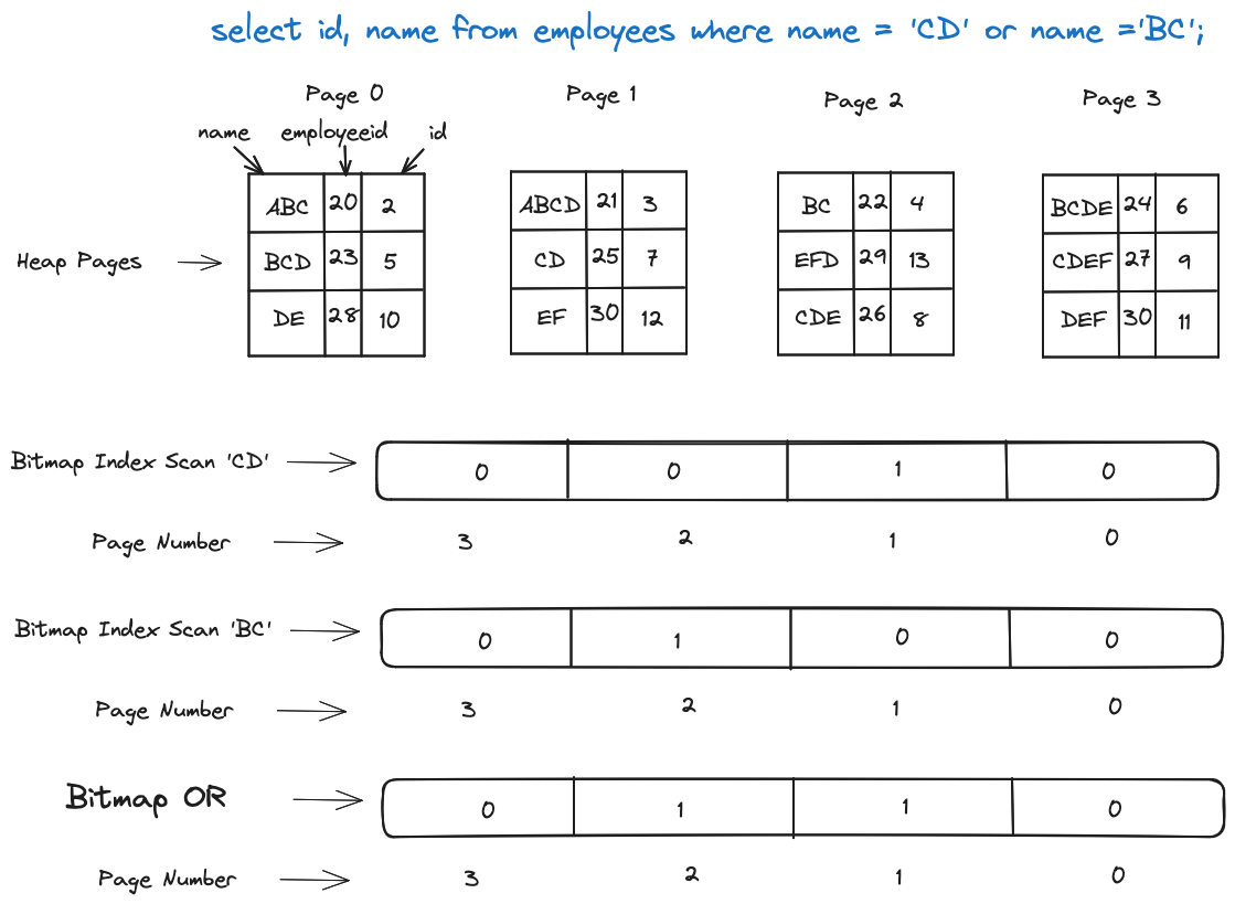
Here's a simplified breakdown of above image:
In a bitmap index scan, rows are not loaded into memory. PostgreSQL sets the bit to 1 for page number 1 when the name is 'CD' and 0 for other pages.
When the name is 'BC', page number 2 is set to 1, and others are set to 0.
Subsequently, a new bitmap is created by performing an OR operation on both bitmaps.
Finally, PostgreSQL executes a Bitmap Heap Scan where it fully scans each heap page and rechecks the conditions.
This approach minimizes the need to load entire pages into memory for individual rows, improving the efficiency of the query. If the query results in a lot of rows located in only a limited number of heap pages then this strategy will be very efficient.
Upon analyzing the provided query, we extract the id and name by applying a filter on the name column, which has an index.
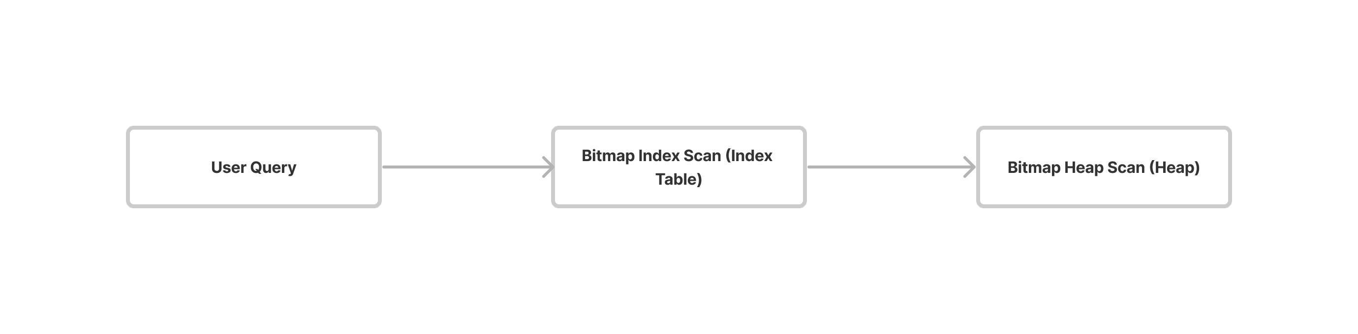
Let's clarify the process:
Bitmap Index Scan: This step involves scanning the index table for the name column since an index exists on it. It retrieves the page number and row number to obtain references to the corresponding records in the heap.
Bitmap Heap Scan: Since we are filtering based on both id and name, this step is necessary to visit the heap and retrieve the values for both attributes for a specific record. The reference to the record is obtained from the preceding Bitmap Index Scan.
Combining Database Indexes
Prerequisite: Let's create a table to learn how to combine indexes.
Here, we can analyze that since we have an index only on column a, a bitmap index scan is performed on column a. To retrieve column c, it jumps to the heap and performs a bitmap heap scan.
Select column c but we are going to query on both a and b with AND operation
This time, Postgres did not use the index numbers_a_b_idx. Even though we have a composite index on both columns a and b. Why? Because we cannot use this composite index when scanning a filter. The filter condition is on column a, and the composite index can be used for conditions involving both columns a and b or just column a. However, it cannot be used for conditions involving only column b. Therefore, if we have a composite index on columns a and b, querying on column b alone will not utilize the index.
Select column c but we are going to query on both A and B with AND operation
As observed earlier, it's not feasible to use a composite index on column B individually. The option is either to use it on column A alone or on both columns A and B. Consequently, Postgres opts for a Parallel Sequential Scan in this scenario.
Manish Sharma
Manish Sharma works in the Technology team at eLitmus and loves building things. Outside of work, he enjoys spending time in nature and swimming.
 Let’s delve into two scenarios:
 Let's break down the query output:

 Here's a simplified breakdown of above image:
 Let's clarify the process: